
Chapter 3: Actor-Critic methods and deep dive into Proximal Policy Optimisation (PPO)

Introduction
Welcome back! Across the first two chapters, we've covered the core concepts of reinforcement learning and explored the fundamental split between value-based and policy-based methods. We learned why policy-based approaches dominate LLM reinforcement learning, but we also saw their limitations - particularly their sample inefficiency and high-variance gradients.
In this chapter, we're picking up exactly where we left off. We'll explore actor-critic methods, which truly deliver the "best of both worlds" we hinted at. Then we'll dive deep into the algorithm that underpins most modern reinforcement learning for LLMs: Proximal Policy Optimization (PPO).
By the end of this chapter, you'll understand not just what PPO does, but why it was needed, how it elegantly solves the instability problems that plagued earlier methods, and why it underpins most of the modern reinforcement learning techniques.
Let's begin!
The Actor-Critic Framework: Bringing Value and Policy Together
Remember our Minesweeper player from the previous chapters? We explored two different learning approaches:
- Value-based: Learn to evaluate how good each tile click is, then act greedily
- Policy-based: Learn clicking patterns directly through trial and error
Actor-critic methods combine both approaches by maintaining two separate but interacting components:
- The Actor (Policy): Decides which actions to take - "I should click this tile"
- The Critic (Value Function): Evaluates how good states or actions are - "This board position looks promising"
Why This Combination matters:
To understand why this pairing is so powerful, let's revisit a key limitation of pure policy methods. In Chapter 2, we introduced the advantage-based policy gradient:
$\nabla_\theta J(\theta) = \mathbb{E}_t\!\left[ \nabla_\theta \log \pi_\theta(a_t \mid s_t)\, \hat{A}_t \right]$
The challenge was computing that advantage estimate $\hat{A}_t$. In pure policy methods, we typically use the simple return: "How much total reward did I get from this point onward?" But this approach is noisy - a single lucky or unlucky outcome can dramatically skew our learning signal.
This is where the critic comes in. Instead of waiting to see what actually happens over an entire game, the critic provides an estimate of expected future value. This allows us to compute much more stable advantage estimates.
The Key Insight: Using Value Functions to Assess Actions
The critical insight behind actor-critic methods lies in how we use value functions to assess actions rather than just states.
Traditional policy methods compute advantages using complete returns - we wait until the end of an episode to see the total reward achieved. But this approach is incredibly noisy. A single lucky break or unfortunate event can skew our entire learning signal.
Actor-critic methods solve this by applying the value function to both the current state and the next state after taking an action. The estimated value of the next state, when discounted and added to the immediate reward, gives us the one-step return:
$G_{t:t+1} = R_{t+1} + \gamma V(S_{t+1})$
This one-step return serves as a much more immediate and less noisy estimate of the actual return, providing a way to assess actions with lower variance.
When the value function is used to assess actions in this way, it's called a critic, and the overall method becomes an actor-critic approach
The Mathematical Foundation
Let’s formalize this. The actor-critic advantage estimate becomes:
$\hat{A}_t = R_{t+1} + \gamma V(S_{t+1}) - V(S_t)$
This is the temporal difference (TD) error - it measures how much better the actual one-step experience was compared to what our value function predicted.
Breaking this down:
- V(S_t): What we expected the current state to be worth
- R_{t+1} + γV(S_{t+1}): What we actually observed (immediate reward plus discounted next state value)
- The difference: How much we were surprised (positively or negatively)
Why Actor-Critic Methods Excel
This combination addresses the key weaknesses of both pure approaches:
From Value-Based Methods, we get:
- Lower variance advantage estimates (thanks to the critic)
- Better sample efficiency through temporal difference learning
From Policy-Based Methods, we get:
- Direct policy optimization for high-dimensional action spaces
- Natural handling of continuous or complex action distributions
The result is a method that's both stable and scalable - exactly what we need for training large language models, which have a large action space.
The Problem with Vanilla Policy Gradients: Understanding Policy Collapse
Before diving into PPO specifically, we need to understand the fundamental stability problem that motivated its development. Let's take a brief but illuminating detour into why vanilla policy gradients often fail catastrophically.
The Fragility of Policy Updates
Recall our basic policy gradient update:
$$\theta \leftarrow \theta + \alpha \nabla_\theta J(\theta)$$
This looks innocent enough - just gradient ascent on our expected reward. But there's a hidden danger in that learning rate $\alpha$.
Imagine our Minesweeper player has learned a decent strategy: it can clear about 60% of a board on average. Now, after one particularly lucky game where it scored +25 points, the policy gradient pushes strongly toward all the actions from that game.
If the learning rate is too large, the updated policy might become radically different from the previous one. The player might suddenly start taking extremely aggressive risks, clicking tiles it would never have considered before
A Functional Analysis Perspective
To really understand this, let's think about the space of all possible policies $\pi$ as points in a high-dimensional function space. The policy gradient is effectively telling us which direction to move in this space to increase expected reward.
The critical insight is that if we move too far - if the step size α is too large - the updated policy $\pi_{\theta_{k+1}}$ might lie "far" from the previous one $\pi_{\theta_k}$. This distance is naturally measured by the Kullback-Leibler divergence:
$D_{KL}(\pi_{\theta_k} \mid \pi_{\theta_{k+1}})$
A high KL divergence means our policy has essentially changed its personality overnight. In Minesweeper terms, a conservative player might suddenly become recklessly aggressive, or vice versa. The policy starts exploring regions of the environment it has no experience with, rendering all prior learning useless.
This is policy collapse - the phenomenon where aggressive policy updates destroy accumulated knowledge and send training into a destructive spiral.
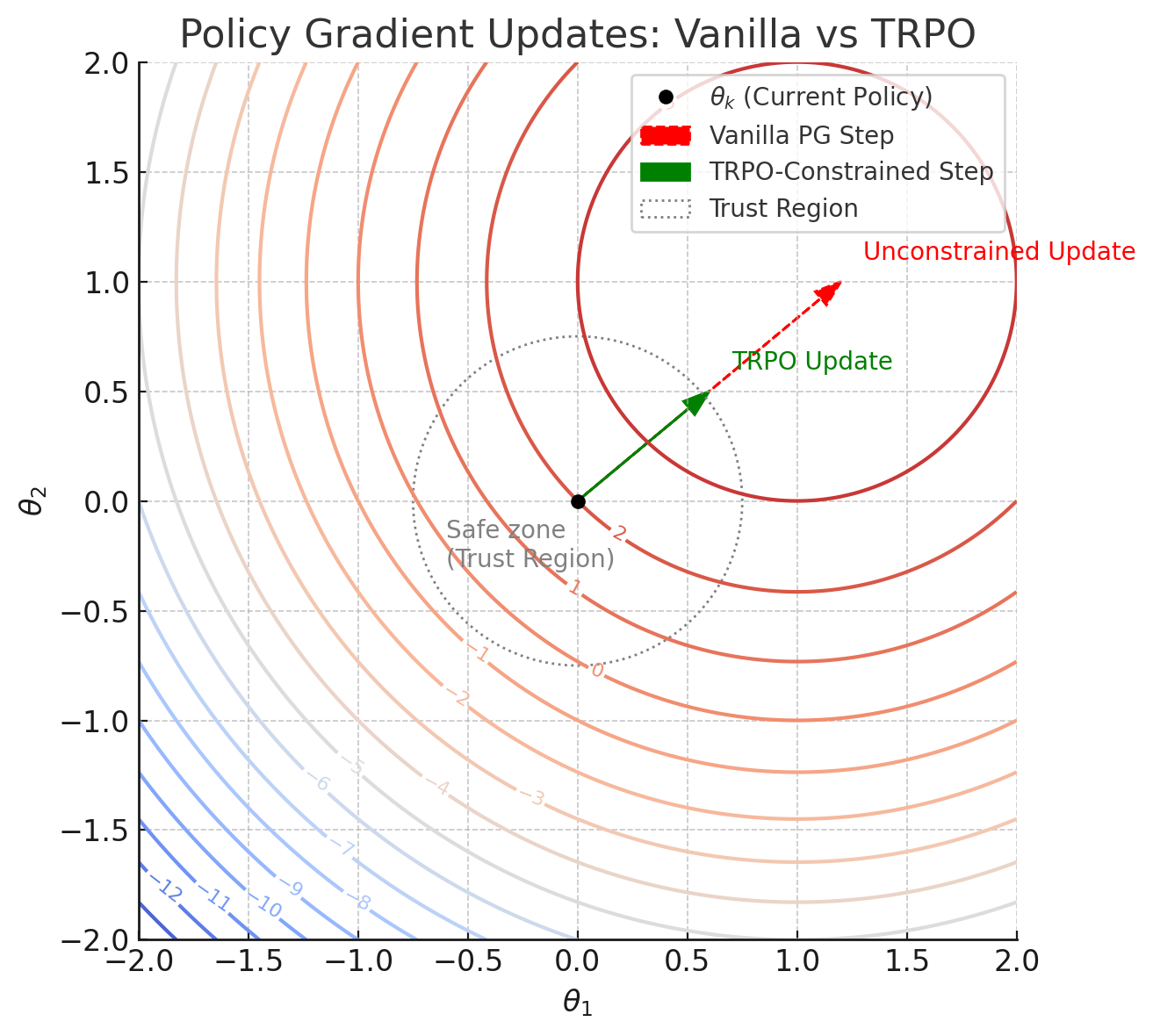
Trust Region Policy Optimization (TRPO): The Principled Fix
Trust Region Policy Optimization emerged as a principled solution to policy collapse. The core idea is beautifully simple: constrain how much the policy can change in each update.
TRPO sets up a constrained optimization problem with two components:
The Objective (what we want to maximize): $L_{CPI}(\theta) = \mathbb{E}_t [r_t(\theta) \hat{A}_t]$
The Constraint (what limits our optimization): $\mathbb{E}_t \left[ D_{KL} \!\left( \pi_{\theta_{\text{old}}}(\cdot \mid s_t) \,\|\, \pi_{\theta}(\cdot \mid s_t) \right) \right] \leq \delta$
Here, $r_t(\theta) = \frac{\pi_\theta(a_t | s_t)}{\pi_{\theta_{old}}(a_t | s_t)}$ is the importance sampling ratio that corrects for the mismatch between the current policy and the policy that generated the data.
These are two separate mathematical entities: the first tells us which direction improves performance, while the second prevents us from moving too far in that direction. The constraint explicitly limits how far each policy can drift in the KL-space, creating a "trust region" of safe updates.
The Computational Challenge
While TRPO's idea was sound, its execution was computationally intensive. To understand just how expensive, let's put this in concrete terms:
Baseline Comparison: A simple policy gradient update requires one forward pass and one backward pass through the neural network - roughly 2N operations where N is the number of parameters. Modern LLMs have billions of parameters, so we're talking about ~4 billion operations per update.
TRPO's Requirements: For each policy update, TRPO must:
- Linear approximation of the objective: This step alone isn't too expensive - another forward pass through the network.
- Quadratic approximation of the constraint: Here's where things get painful. Computing the KL divergence constraint requires computing the Hessian (matrix of second-order derivatives) of the KL divergence with respect to all policy parameters.
Let's make this concrete. Imagine our policy has just 1 million parameters (tiny by modern standards). The Hessian is a 1M × 1M matrix - that's 1 trillion entries to compute and store. For a model like GPT-3 with 175 billion parameters, we'd need a matrix with roughly 30,000 trillion trillion entries!
- Conjugate gradient descent: To find the optimal update direction while respecting the constraint, TRPO must solve a system of linear equations involving this massive Hessian matrix. This typically requires 10-20 iterations of conjugate gradient, each involving matrix-vector products with the Hessian.
- Line search: Finally, TRPO performs a series of trial policy evaluations to find the largest step size that doesn't violate the trust region constraint. This means computing multiple forward passes and checking the KL constraint each time.
The Reality Check: While vanilla policy gradients might complete an update in seconds, TRPO could take hours or even days for large models. The memory requirements alone make it impractical - storing a Hessian matrix for a billion-parameter model would require petabytes of memory.
In short: brilliant idea, but prohibitively expensive for large-scale applications.
Enter PPO: Stable, Scalable, Simple
Proximal Policy Optimization (PPO) addresses TRPO's computational overhead while maintaining its stability benefits. The key insight: instead of explicitly constraining the KL divergence, why not build the constraint directly into the objective function?
The Clipped Surrogate Objective
PPO's central innovation is the clipped surrogate objective:
$$L^{CLIP}(\theta) = \mathbb{E}_t\left[ \min \left(r_t(\theta) \hat{A}_t, \text{clip}(r_t(\theta), 1 - \epsilon, 1 + \epsilon) \hat{A}_t \right) \right]$$
Where $r_t(\theta) = \frac{\pi_\theta(a_t | s_t)}{\pi_{\theta_{old}}(a_t | s_t)}$ is the probability ratio, and $\epsilon$ is a hyperparameter (typically 0.2).
Let's unpack why this is brilliant:
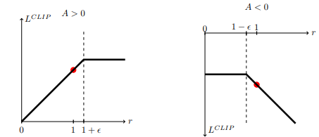
Case 1: Positive Advantage ($\hat{A}_t > 0$)
When an action was better than expected, we want to increase its probability. The objective becomes:
$$\min(r_t(\theta) \hat{A}_t, (1 + \epsilon)\hat{A}_t)$$
As $r_t(\theta)$ increases (meaning we're making the good action more likely), the term $r_t(\theta) \hat{A}_t$ grows. But once it hits the threshold $(1 + \epsilon)$, the gradient becomes zero - there's no incentive to push further.
In Minesweeper terms: if clicking a particular tile pattern worked well, we'll increase its probability, but only up to a reasonable limit. We won't become obsessively fixated on that pattern.
Case 2: Negative Advantage ($\hat{A}_t < 0$)
When an action was worse than expected, we want to decrease its probability. The objective becomes:
$$\min(r_t(\theta) \hat{A}_t, (1 - \epsilon)\hat{A}_t)$$
Since $\hat{A}_t$ is negative, the min operation selects the more negative value. If $r_t(\theta)$ drops below $(1 - \epsilon)$, the gradient is clipped, capping the penalty.
Why Clipping Works
This clipping mechanism elegantly prevents the policy from changing too dramatically in either direction:
- For good actions: We increase their probability, but not excessively
- For bad actions: We decrease their probability, but don't eliminate them entirely
The beauty is that this achieves TRPO's stability guarantees using only first-order optimization - no second derivatives, no complex constrained optimization, just straightforward gradient ascent (which we all know and love 😀)
The Complete PPO Algorithm
While the clipped objective is PPO's star feature, the complete algorithm operates within an actor-critic framework with several additional components:
The Full Objective Function
$$L_{\text{total}}(\theta) = L_{\text{CLIP}}(\theta) - c_1 L_{\text{VF}}(\phi) + c_2 H[\pi_{\theta}]$$
Let's break down each term:
1. The Clipped Surrogate Objective ($L_{\text{CLIP}}$): Our main policy improvement signal
2. The Value Function Loss ($L_{\text{VF}}$): Trains the critic to better estimate state values $L_{\text{VF}}(\phi) = \mathbb{E}_t \left[ \big(V_{\phi}(s_t) - V_t^{\text{target}}\big)^2 \right]$
3. The Entropy Bonus ($H[\pi_{\theta}]$): Encourages exploration by rewarding policy uncertainty $H[\pi_{\theta}] = \mathbb{E}_t \left[ - \log \pi_\theta(a_t \mid s_t) \right]$
The coefficients $c_1$ and $c_2$ balance the relative importance of value learning and exploration against the main policy objective.
The Role of Entropy
The entropy bonus deserves special attention. Without it, successful policies might become overconfident, always choosing the same actions in given states. This eliminates exploration and can lead to getting stuck in local optima.
High entropy means the policy is "curious" - willing to try different actions. Low entropy means it's "decisive" (or deterministic, in formal speak) - consistently choosing particular actions. The entropy bonus provides a knob to tune this exploration-exploitation tradeoff.
The Training Loop
PPO's training procedure brings all these pieces together:
- Collect Trajectories: Roll out the current policy in the environment to gather experience
- Compute Targets: Calculate advantages using Generalized Advantage Estimation (GAE)
- Optimize: Perform multiple epochs of minibatch SGD on the combined objective
- Update: Set $\theta_{\text{old}} \leftarrow \theta$ and repeat
The multi-epoch training on each batch of data helps improve sample efficiency - unlike vanilla policy gradients that use each experience only once.
A Minimal PyTorch Implementation
To make these concepts concrete, here’s a rather simplified PyTorch implementation of the code PPO update:
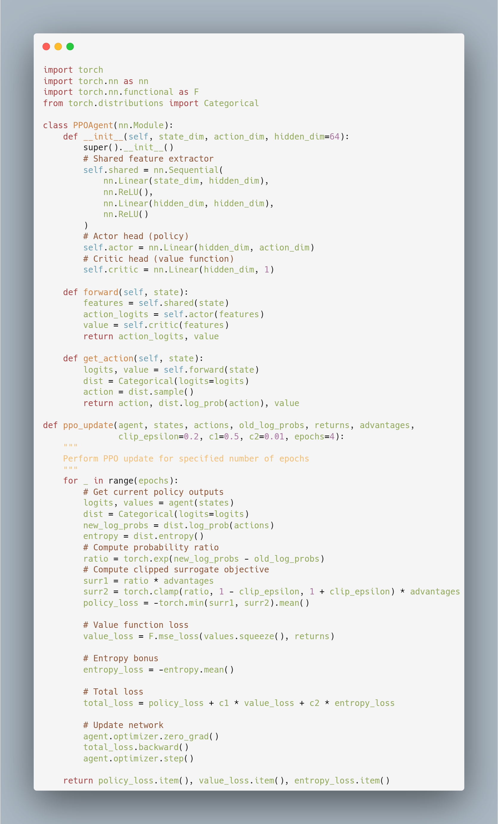
This implementation captures all of PPO's essential components:
- Shared network architecture: Common feature extraction for both actor and critic
- Clipped surrogate objective: The torch.clamp operation implements the crucial clipping mechanism
- Multi-epoch training: The outer loop allows reusing experience data multiple times
- Combined loss: Balances policy improvement, value learning, and exploration
While this is simplified compared to production implementations (which include additional optimizations like gradient clipping, learning rate scheduling, and more sophisticated advantage estimation), it demonstrates how PPO's theoretical insights translate into practical code.
A Note on Generalized Advantage Estimation (GAE)
PPO typically uses GAE for computing advantage estimates, which balances bias and variance by mixing different temporal difference lengths:
$\hat{A}_t^{\text{GAE}(\gamma,\lambda)} = \sum_{l=0}^{\infty} (\gamma \lambda)^l \delta_{t+l}$
Where $\delta_t = r_t + \gamma V(s_{t+1}) - V(s_t)$ is the temporal difference error.
This provides more stable advantage estimates than simple one-step TD errors, further improving training stability. There is significantly more to this algorithm than what we’ve covered, however, covering it in depth would be beyond the scope of this blog. For the more inclined, you can read about GAE here
Why PPO Became the Bedrock for Modern RL Algorithms
PPO struck a rare balance in the RL world:
Simplicity: First-order optimization, no complex constrained optimization procedures Stability: Clipping prevents policy collapse without requiring explicit KL constraints
Scalability: Efficient enough for large-scale applications like LLM training Effectiveness: Consistently good performance across diverse environments
These qualities made PPO the natural choice when the field turned toward training large language models with reinforcement learning. Famously, GPT-3’s Instruct variant was optimized using PPO - which was much better at following human instructions than its pretrained counterpart.
PPO in LLM Training: From Minesweeper to Language
When we move from Minesweeper to language modeling, the core PPO algorithm remains the same, but the mapping changes:
- State: The current sequence of tokens generated so far
- Action: Choosing the next token from the vocabulary
- Policy: The language model's probability distribution over next tokens
- Reward: Human feedback, helpfulness scores, or other alignment signals
- Advantage: How much better a particular token choice was compared to the model's typical behavior
The clipping mechanism becomes crucial in language settings because token choices can be highly sensitive - a single token can completely change the meaning of a response. PPO ensures that the model evolves gradually toward more helpful behavior without losing its basic language capabilities.
Looking Forward
PPO represents a pivotal moment in reinforcement learning - the point where theoretical rigor met practical scalability. It solved the stability problems that plagued earlier policy methods while remaining computationally feasible for large-scale applications.
But PPO is not the end of the story. Modern variants like GRPO (Group Relative Policy Optimization) have emerged that challenge some of PPO's assumptions, particularly the need for a separate critic (which also induces a lot of computational overhead for bigger models) network. Algorithms like Dynamic Sampling Policy Optimization (DAPO) and Group Sequence Policy Optimization (GSPO) try to address the flaws in GRPO - which we’ll discuss in the next chapter.
In our next chapter, we'll explore these modern alternatives, starting with GRPO's radical departure from the actor-critic framework. We'll see how recent innovations are pushing the boundaries of what's possible in LLM training, building on PPO's solid foundation while addressing its remaining limitations.
Stay tuned for more informative blogs 😀